Flow Fields
A flow field is a grid of vectors. It essentially defines a path. And it is one of my favorite techniques for creating generative art.
What is Flow (Vector) Field
A vector field is a function that assigns each point to the vector . In physics, it helps to visualize and understand gravitation and electromagnetism. But in this article, we are not interested in those.
If we think about mathematics, we can define a vector field function like this:
In programming, I divide flow fields into two parts. Parametric flow fields and non-parametric flow fields.
Parametric flow fields are fields that can be described using mathematical functions, such as , , etc. Non-parametric flow fields are opposite of the above. One and probably the most popular example could be a noise field. We will discuss (and create) both flow fields later on.
Creating Flow Field
Creating a flow field is the same for all programming languages. I am using TypeScript and the p5.js library in this article. You can use your preferred programming language and the library. It doesn't matter as long as you understand the logic behind it.
Generally, both parametric and non-parametric flow fields are created using floating-point numbers in the range. But we need vectors. So how do we convert these numbers to vectors, by using angles.
We need a function that takes a number and returns an angle. Since I am using p5.js, there is a beautiful function called map() in p5. Full function
definition is something like this;
map(value, oldMin, oldMax, newMin, newMax) => number;map(value, oldMin, oldMax, newMin, newMax) => number;For example, calling map(0.5, 0, 1, 0, 360) returns 180. It changes the value's range.
Now, we have all the background for creating a flow field. Let's start by creating parametric flow fields.
Parametric Flow Field
So, we need a function. For the sake of simplicity, I am going to use my beloved function. To be exact, I am going to use . If you noticed,
this function is not returning a vector, it returns a scalar. That is because we want to create a vector from this function by using map.
Let's start coding by creating a JavaScript file and creating a flow field function.
function f(x, y) {
  return sin(x) + cos(y);
}
function f(x, y) {
return sin(x) + cos(y);
}We don't actually want a function like that because of its range. and functions have a range of . Adding these two ranges yields .
If we divide this range by 2, then we would have which is great for our function. So let's change out the f function.
function f(x, y) {
  return (sin(x) + cos(y)) * 0.5;
}
function f(x, y) {
return (sin(x) + cos(y)) * 0.5;
}Since we want to convert this number to angle, we also need to map this result to range .
function f(x, y) {
  const value = (sin(x) + cos(y)) * 0.5;
  return map(value, -1, 1, 0, TWO_PI);
}
function f(x, y) {
const value = (sin(x) + cos(y)) * 0.5;
return map(value, -1, 1, 0, TWO_PI);
}So, this is our parametric flow field function. Now we can visualize what it looks like. For simplicity, I am going to use lines to visualize.
Let's start by creating some p5.js functions.
function setup() {
createCanvas(500, 500);
background(255);
noLoop();
}
function draw() {}function setup() {
createCanvas(500, 500);
background(255);
noLoop();
}
function draw() {}To not burn my computer, I am also going to create a constant called RESOLUTION. This will be used while getting numbers for our flow field. Let's start by filling
our draw function.
function draw() {
for (let x = RESOLUTION / 2; x < width; x += RESOLUTION) {
for (let y = RESOLUTION / 2; y < height; y += RESOLUTION) {
const angle = f(x, y);
line(x, y, x + 10 * cos(angle), y + 10 * sin(angle));
}
}
}function draw() {
for (let x = RESOLUTION / 2; x < width; x += RESOLUTION) {
for (let y = RESOLUTION / 2; y < height; y += RESOLUTION) {
const angle = f(x, y);
line(x, y, x + 10 * cos(angle), y + 10 * sin(angle));
}
}
}The full code looks something like this:
const RESOLUTION = 25;
function f(x, y) {
  const value = (sin(x) + cos(y)) * 0.5;
  return map(value, -1, 1, 0, TWO_PI);
}
function setup() {
createCanvas(500, 500);
background(255);
noLoop();
}
function draw() {
  for (let x = RESOLUTION / 2; x < width; x += RESOLUTION) {
    for (let y = RESOLUTION / 2; y < height; y += RESOLUTION) {
      const angle = f(x, y);
      line(x, y, x + 10 * cos(angle), y + 10 * sin(angle));
    }
  }
}const RESOLUTION = 25;
function f(x, y) {
const value = (sin(x) + cos(y)) * 0.5;
return map(value, -1, 1, 0, TWO_PI);
}
function setup() {
createCanvas(500, 500);
background(255);
noLoop();
}
function draw() {
  for (let x = RESOLUTION / 2; x < width; x += RESOLUTION) {
    for (let y = RESOLUTION / 2; y < height; y += RESOLUTION) {
      const angle = f(x, y);
      line(x, y, x + 10 * cos(angle), y + 10 * sin(angle));
    }
  }
}These for loops are self-explanatory, we are just looping through every grid cell. Inside both loops, we are calling the flow field function with current x and y positions.
Remember, this function returns a radian. Radians are useful because polar coordinates are great for angles. We also can convert from polar coordinate-system to cartesian
coordinate-system easily.
cos(angle) means we want the angle's projection to x-axes. Meaning that it returns the x value of the point.
sin(angle) is the same thing but returns the y value of the point.
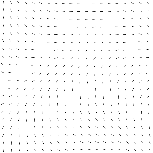
We are multiplying these conversions by 10 (or any number) to change their length. If we run this code, we should see something like this.

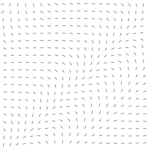
Here is another parametric flow field defined by the function

Non-parametric Flow Field
Non-parametric flow fields can't be expressed as mathematical functions. One example is noise flow fields. In this article, we are going to create a non-parametric flow field using noise. Let's start by creating a function that returns a noise value for given x and y.
function f(x, y) {
  return noise(x, y);
}
function f(x, y) {
return noise(x, y);
}In p5, the noise function has a range . This means we can directly use this value for our map function.
function f(x, y) {
  const value = noise(x, y);
  return map(value, 0, 1, 0, TWO_PI);
}
function f(x, y) {
const value = noise(x, y);
return map(value, 0, 1, 0, TWO_PI);
}Now, our function returns a value between which is radian. The rest is the same. So the full code looks something like this:
const RESOLUTION = 25;
function f(x, y) {
  const value = noise(x, y);
  return map(value, 0, 1, 0, TWO_PI);
}
function setup() {
createCanvas(500, 500);
background(255);
noLoop();
}
function draw() {
for (let x = RESOLUTION / 2; x < width; x += RESOLUTION) {
for (let y = RESOLUTION / 2; y < height; y += RESOLUTION) {
const angle = f(x, y);
line(x, y, x + 10 * cos(angle), y + 10 * sin(angle));
}
}
}const RESOLUTION = 25;
function f(x, y) {
const value = noise(x, y);
return map(value, 0, 1, 0, TWO_PI);
}
function setup() {
createCanvas(500, 500);
background(255);
noLoop();
}
function draw() {
for (let x = RESOLUTION / 2; x < width; x += RESOLUTION) {
for (let y = RESOLUTION / 2; y < height; y += RESOLUTION) {
const angle = f(x, y);
line(x, y, x + 10 * cos(angle), y + 10 * sin(angle));
}
}
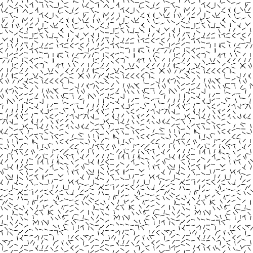
}If we run this, we should get something chaotic like this:

This is because the noise function returns values far apart from each other. To fix this issue, we can multiply x and y arguments by a small number to change the 'scale' of the noise.
In the f function, let's multiply x and y arguments by 0.001.
function f(x, y) {
  const value = noise(x * 0.001, y * 0.001);
  return map(value, 0, 1, 0, TWO_PI);
}
function f(x, y) {
const value = noise(x * 0.001, y * 0.001);
return map(value, 0, 1, 0, TWO_PI);
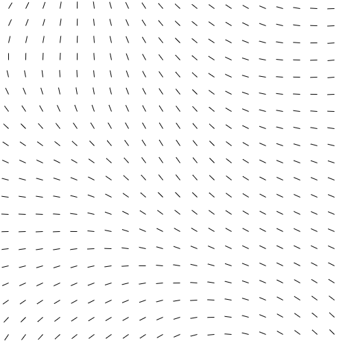
}If we run again, we should see a less chaotic noise flow field, something like below.

It looks like a parametric flow field but every time we re-run the code, we see different output. That is the beauty and generativeness of non-parametric flow fields (especially the noise).
After creating flow fields, we should think about how to visualize them. There are several techniques for visualizing flow fields. Actually, we already learned one of them, we just drew lines according to the angle of the flow field. Other ways could be simulating little particles or moving shapes according to the flow fields.
Conclusion
So, yeah. I tried my best to explain flow and vector fields.
Hopefully, this article has created something in your mind about flow fields. My advice is to try different things with flow fields. Try to change parameters, try different visualization techniques. Understanding flow fields is I think just the tip of the iceberg.
Until next time and thanks for reading.